Contents
- Definition & Structure
- Reconstructions
- Probability Distributions
- Parameters & k
- Continuous RBMs
- Next Steps
- Other Resources
Definition & Structure
In 2024, Geoffrey Hinton received the Nobel Prize in Physics for his work on Restricted Boltzmann Machines. Congrats, Geoff!
Invented by Geoffrey Hinton, a Restricted Boltzmann machine is an algorithm useful for dimensionality reduction, classification, regression, collaborative filtering, feature learning and topic modeling.
Given their relative simplicity and historical importance, restricted Boltzmann machines are the first neural network we’ll tackle. In the paragraphs below, we describe in diagrams and plain language how they work.
RBMs are shallow, two-layer neural nets that constitute the building blocks of deep-belief networks. The first layer of the RBM is called the visible, or input, layer, and the second is the hidden layer. (Editor’s note: While RBMs are occasionally used, most practitioners in the machine-learning community have deprecated them in favor of generative adversarial networks or variational autoencoders. RBMs are the Model T’s of neural networks – interesting for historical reasons, but surpassed by more up-to-date models.)
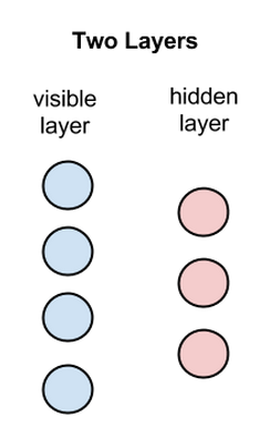
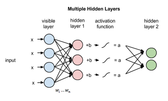
Each circle in the graph above represents a neuron-like unit called a node, and nodes are simply where calculations take place. The nodes are connected to each other across layers, but no two nodes of the same layer are linked.
That is, there is no intra-layer communication: this is the restriction in a restricted Boltzmann machine. In a binary RBM, each unit has a state of zero or one. During sampling, it turns on with a probability determined by the other layer’s states, the connecting weights and its bias. This sampling makes the units stochastic.
Each visible node takes a low-level feature from an item in the dataset to be learned. For example, from a dataset of grayscale images, each visible node would receive one pixel-value for each pixel in one image. (MNIST images have 784 pixels, so neural nets processing them must have 784 input nodes on the visible layer.)
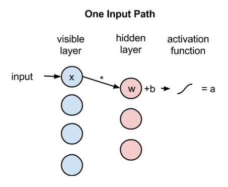
Now let’s follow that single pixel value, x, through the two-layer net. At node 1 of the hidden layer, x is multiplied by a weight and added to a bias. For a binary hidden unit, applying the sigmoid function gives its probability of turning on. We can then sample a zero-or-one state from that probability.
probability of a = 1: sigmoid((weight w * input x) + bias b)
Next, let’s look at how several inputs combine at one hidden node. Each x is multiplied by a separate weight. We sum those products, add the node’s bias and apply the sigmoid to get its activation probability.
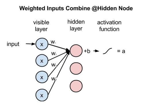
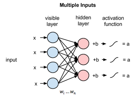
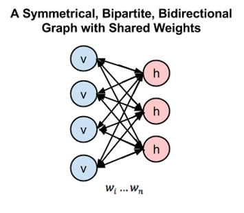
Because inputs from all visible nodes are being passed to all hidden nodes, an RBM can be defined as a symmetrical bipartite graph.
Symmetrical means that the same connection weight is used when computing either layer’s probabilities from the other. Bipartite means the graph has two groups of nodes, with connections only between groups. Here, every visible node connects to every hidden node.
At each hidden node, each input x is multiplied by its respective weight w. That is, a single input x would have three weights here, making 12 weights altogether (4 input nodes x 3 hidden nodes). The weights between two layers will always form a matrix where the rows are equal to the input nodes, and the columns are equal to the output nodes.
Each hidden node receives the four inputs multiplied by their respective weights. Its bias shifts the probability of activation: a larger bias makes the node more likely to turn on for the same input. It does not guarantee that any node will turn on.
RBMs can be trained in a stack. The first RBM’s hidden activations supply the data for a second RBM, which learns another representation. These learned weights can later initialize a deeper classifier or autoencoder.
Reconstructions
An RBM learns a probability distribution over its inputs. Training aims to assign higher probability to examples in the training data. This can be unsupervised: the examples need no class labels. Reconstructions appear during training because the model alternates between sampling hidden states from visible states and visible states from hidden states.
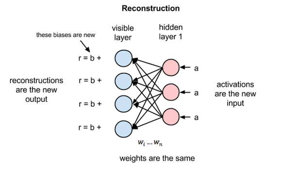
To reconstruct a binary input, first sample hidden states from their activation probabilities. For each visible unit, sum the weighted hidden states, add its visible bias and apply the sigmoid. This gives the probability of that visible unit being one. Sampling those visible units produces a reconstruction. The same connection weights work in both directions:
The learning signal compares how often a visible unit and a hidden unit are active together under two conditions: when the visible layer holds training data, and when the network samples from its own model distribution. These are called the positive and negative statistics. Increasing a connection’s weight favors that pair being active together. The update strengthens pairs that occur more often with the data than the model currently predicts.
Sampling accurately from the model can be slow. Contrastive divergence, or CD, approximates the second set of statistics with a short sampling chain started at a training example. In CD-1, we sample hidden states from that example, reconstruct the visible states, then compute hidden probabilities from the reconstruction. The weight update uses the difference between the original and reconstructed visible-hidden associations. This is a biased approximation to the log-likelihood gradient. Hinton, Osindero and Teh describe the learning rule in section 3 of their paper.
Pixel-by-pixel reconstruction error is a useful diagnostic, but CD does not backpropagate that error through the RBM. Low reconstruction error can coexist with a poor model of the data. Hinton’s practical guide explains this limitation in section 5.
Using x for visible states and a for hidden states, the two sampling directions are p(a|x) and p(x|a). The weights and biases define a joint distribution p(x, a) from which both conditional distributions follow.
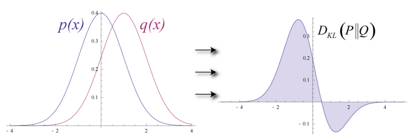
Fitting a distribution to the data is called generative learning. Maximum-likelihood training is equivalent to minimizing the Kullback–Leibler divergence from the empirical data distribution p to the model distribution q. For discrete inputs, KL(p || q) = sum_x p(x) log(p(x) / q(x)). This weights each log probability ratio by how often that input occurs in the data. Hinton’s contrastive-divergence paper develops this connection.
The following curves illustrate two continuous distributions. On the right, the signed area under p(x) log(p(x) / q(x)) gives their KL divergence. It is not the non-overlapping area between the curves.
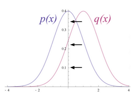
The next picture illustrates a model distribution approaching a data distribution. It is a sketch of the fitting goal; individual CD updates need not reduce KL divergence, and the distributions need not be bell curves.
Probability Distributions
Let’s talk about probability distributions for a moment. If you’re rolling two dice, the probability distribution for all outcomes looks like this:
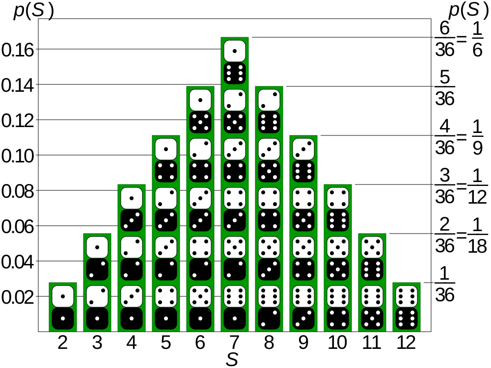
That is, 7s are the most likely because there are more ways to get to 7 (3+4, 1+6, 2+5) than there are ways to arrive at any other sum between 2 and 12. Any formula attempting to predict the outcome of dice rolls needs to take seven’s greater frequency into account.
Or take another example: Languages are specific in the probability distribution of their letters, because each language uses certain letters more than others. In English, the letters e, t and a are the most common, while in Icelandic, the most common letters are a, r and n. Attempting to reconstruct Icelandic with a weight set based on English would lead to a large divergence.
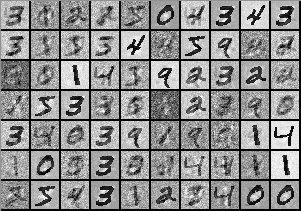
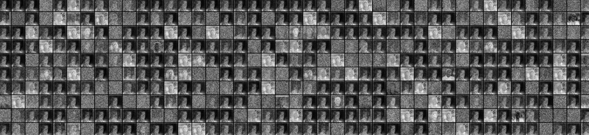
In the same way, image datasets have unique probability distributions for their pixel values, depending on the kind of images in the set. Pixels values are distributed differently depending on whether the dataset includes MNIST’s handwritten numerals:
or the headshots found in Labeled Faces in the Wild:
Imagine an RBM fed images of elephants and dogs. Its hidden units might learn patterns involving trunks, ears or fur, without receiving animal labels. Given the pixels, it samples a combination of hidden features. Given those hidden states, it samples a possible arrangement of pixels.
The joint probability p(x, a) describes the probability of a particular visible pattern and hidden state occurring together.
The process of learning reconstructions is, in a sense, learning which groups of pixels tend to co-occur for a given set of images. The activations produced by nodes of hidden layers deep in the network represent significant co-occurrences; e.g. “nonlinear gray tube + big, floppy ears + wrinkles” might be one.
In the two images above, you see reconstructions learned by Deeplearning4j’s implementation of an RBM. They show what the hidden states can reconstruct. Inspecting these images can reveal problems such as units that stay on for every input, but recognizable reconstructions alone do not establish that the model assigns sensible probabilities to new data.
Each hidden and visible unit has its own bias. Hidden biases affect which features activate; visible biases affect which input values the model tends to generate. Both sets of biases are learned alongside the shared weights.
Multiple Layers
Once this RBM learns the structure of the input data as it relates to the activations of the first hidden layer, then the data is passed one layer down the net. Your first hidden layer takes on the role of visible layer. The activations now effectively become your input, and they are multiplied by weights at the nodes of the second hidden layer, to produce another set of activations.
This process of creating sequential sets of activations by grouping features and then grouping groups of features is the basis of a feature hierarchy, by which neural networks learn more complex and abstract representations of data.
Each RBM is trained on the representation supplied by the previous one. This is greedy, layerwise and unsupervised pre-training: it learns one pair of layers at a time, using unlabeled examples.
Because those weights already approximate the features of the data, they are well positioned to learn better when, in a second step, you try to classify images with the deep-belief network in a subsequent supervised learning stage.
Pre-training can provide starting weights for a later stage that uses backpropagation. In a classifier, that stage can optimize a label-based loss. In Hinton and Salakhutdinov’s deep autoencoder, backpropagation fine-tunes reconstruction after RBM pre-training. The reconstruction-loss training belongs to that later autoencoder stage.
To synthesize restricted Boltzmann machines in one diagram, here is a symmetrical bipartite and bidirectional graph:
For those interested in studying the structure of RBMs in greater depth, they are one type of undirectional graphical model, also called markov random field.
Parameters & k
In CD-k, k counts full alternating Gibbs-sampling steps before collecting the negative statistics for a weight update. Each step samples the hidden layer given the visible layer, then the visible layer given the hidden layer. Hidden probabilities are computed once more from the final visible sample to measure its associations.
CD-1 uses one such step. Larger values give the sampling chain more time to explore, at greater computational cost. They do not count training epochs or repeated backpropagation passes.
Legacy implementations such as Deeplearning4j exposed settings with names like the following. The unit types determine the probabilities and sampling rules used by the RBM.
weightInit, or weightInitialization represents the starting value of the coefficients that amplify or mute the input signal coming into each node. Proper weight initialization can save you a lot of training time, because training a net is nothing more than adjusting the coefficients to transmit the best signals, which allow the net to classify accurately.
activationFunction determines how a weighted input becomes an activation. For a binary RBM unit, the sigmoid gives a probability; a separate sampling step determines the unit’s state.
optimizationAlgo selects the optimizer used by a particular training routine. L-BFGS is a limited-memory quasi-Newton method: it approximates curvature from successive changes in parameters and gradients, without computing second derivatives directly. This optimizer setting is separate from how CD estimates an RBM’s learning signal.
regularization methods such as l2 help fight overfitting in neural nets. Regularization essentially punishes large coefficients, since large coefficients by definition mean the net has learned to pin its results to a few heavily weighted inputs. Overly strong weights can make it difficult to generalize a net’s model when exposed to new data.
VisibleUnit/HiddenUnit refers to the layers of a neural net. The VisibleUnit, or layer, is the layer of nodes where input goes in, and the HiddenUnit is the layer where those inputs are recombined in more complex features. Both units have their own so-called transforms, in this case Gaussian for the visible and Rectified Linear for the hidden, which map the signal coming out of their respective layers onto a new space.
lossFunction may specify a reported reconstruction metric or the objective for later fine-tuning. A setting such as SQUARED_ERROR does not turn CD training into backpropagation of reconstruction error. Check which training stage an implementation applies it to.
learningRate, like momentum, affects how much the neural net adjusts the coefficients on each iteration as it corrects for error. These two parameters help determine the size of the steps the net takes down the gradient towards a local optimum. A large learning rate will make the net learn fast, and maybe overshoot the optimum. A small learning rate will slow down the learning, which can be inefficient.
Continuous RBMs
A continuous restricted Boltzmann machine is a form of RBM that accepts continuous input (i.e. numbers cut finer than integers) via a different type of contrastive divergence sampling. This allows the CRBM to handle things like image pixels or word-count vectors that are normalized to decimals between zero and one.
It should be noted that every layer of a deep-learning net requires four elements: the input, the coefficients, a bias and the transform (activation algorithm).
The input is a numeric vector, supplied by the previous layer or the original data. The weights and biases determine each unit’s conditional distribution. The unit type specifies how values are sampled from that distribution.
Those additional algorithms and their combinations can vary layer by layer.
An effective continuous restricted Boltzmann machine employs a Gaussian transformation on the visible (or input) layer and a rectified-linear-unit transformation on the hidden layer. That’s particularly useful in facial reconstruction. For RBMs handling binary data, simply make both transformations binary ones.
Gaussian transformations do not work well on RBMs’ hidden layers. The rectified-linear-unit transformations used instead are capable of representing more features than binary transformations, which we employ on deep-belief nets.
Conclusions & Next Steps
For binary visible units, reconstruction probabilities lie between zero and one. A value of 0.8 means an 80% chance of that unit being on, given the hidden states. Nonzero values alone provide no evidence of successful training. Gaussian visible units instead produce real-valued samples or means, which are not percentages.
It should be noted that RBMs do not produce the most stable, consistent results of all shallow, feedforward networks. In many situations, a dense-layer autoencoder works better. Indeed, the industry is moving toward tools such as variational autoencoders and GANs.