Contents
- Neural Network Definition
- A Few Concrete Examples
- Neural Network Elements
- What Makes Learning Deep?
- Example: Feedforward Networks
- Multiple Linear Regression
- Activation Functions
- Crop Yield Through Two Hidden Layers
- Gradient Descent
- Logistic Regression & Classifiers
- Neural Networks & Artificial Intelligence
Neural Network Definition
A neural network is a model that learns to transform numerical inputs into useful outputs by adjusting weights and biases. For an image, the inputs might be pixel values; for a crop, they might describe fertilizer and weather. Its output could be a category probability or a continuous prediction such as yield.
The intermediate layers learn representations, sets of features computed from the input. Those features can support classification, regression, or another algorithm that groups similar examples. The training objective determines which features the network has an incentive to learn.
What kind of problems does deep learning solve, and more importantly, can it solve yours? To know the answer, you need to ask a few questions:
-
What outcomes do I care about? In a classification problem, those outcomes are labels that could be applied to data: for example,
spamornot_spamin an email filter,good_guyorbad_guyin fraud detection,angry_customerorhappy_customerin customer relationship management. Other types of problems include anomaly detection (useful in fraud detection and predictive maintenance of manufacturing equipment), and clustering, which is useful in recommendation systems that surface similarities. -
Do I have the right data? For example, if you have a classification problem, you’ll need labeled data. Is the dataset you need publicly available, or can you create it (with a data annotation service like Scale or AWS Mechanical Turk)? In this example, spam emails would be labeled as spam, and the labels would enable the algorithm to map from inputs to the classifications you care about. You can’t know that you have the right data until you get your hands on it. If you are a data scientist working on a problem, you can’t trust anyone to tell you whether the data is good enough. Only direct exploration of the data will answer this question.
A Few Concrete Examples
A neural network learns a mapping from inputs to outputs. The examples below differ in what those outputs represent and in how we measure whether they are useful.
Classification
In supervised classification, training examples pair inputs with category labels. Labels can come from human annotation or recorded outcomes. The network learns to assign probabilities to those categories. See supervised learning.
- Detect faces, identify people in images, recognize facial expressions (angry, joyful)
- Identify objects in images (stop signs, pedestrians, lane markers…)
- Recognize gestures in video
- Detect voices, identify speakers, transcribe speech to text, recognize sentiment in voices
- Classify text as spam (in emails), or fraudulent (in insurance claims); recognize sentiment in text (customer feedback)
Whether these predictions are useful depends on the quality of the labels and how well the training examples represent the conditions where the model will be used.
Clustering
Clustering groups examples according to a measure of similarity. A neural network can learn numerical representations that a clustering algorithm then uses to group related images or documents. Unsupervised learning learns from data without supplied target labels; the choice of objective still determines what kinds of similarity a representation captures.
- Search: Comparing documents, images or sounds to surface similar items.
- Anomaly detection: The flipside of detecting similarities is detecting anomalies, or unusual behavior. In many cases, unusual behavior correlates highly with things you want to detect and prevent, such as fraud.
Regression: Predicting a Quantity
Regression predicts a continuous value, such as a crop’s yield or a building’s electricity consumption. Forecasting applies such a prediction to a future observation. The distinction between regression and classification is the kind of target, rather than whether the prediction concerns the future.
The crop example below uses fertilizer, sunlight and rainfall to predict tonnes harvested per hectare. Its final layer produces a number in those units.
Neural Network Elements
A layer contains units, also called nodes. In a dense layer, each unit multiplies its input values by weights, adds the products and a bias, then applies an activation function. The bias provides an adjustable offset; the activation determines how the summed signal is transformed.
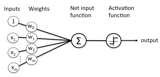
An activation can produce a continuous value. A layer collects its units’ activations into a vector that becomes the next layer’s input. The dense-layer definition formalizes this calculation.
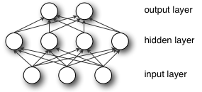
Training adjusts the weights and biases so that these intermediate representations help reduce the chosen loss. A unit’s coefficients control how its inputs contribute to the weighted sum.
What Makes Learning Deep?
Deep learning trains neural networks with multiple layers of learned representations. Each layer transforms the preceding layer’s output, giving the next layer a different description of the same input. The intermediate layers are called hidden layers because their values are computed inside the network, between its inputs and final output.
In an image model, early layers may respond to edges. Later layers can combine those responses into shapes useful for recognizing an object. This is a feature hierarchy: the network builds representations from other representations. Training adjusts the weights that create them, often across the whole network together.
Depth describes the succession of transformations along a path through the network. Width describes how many units a layer contains. A network with two hidden layers is a small example of deep learning; the crop-yield calculation below follows every value through one. Adding layers gives the model more stages for combining features, while also creating more computations to train and check against new data.
Architecture names describe different choices. Convolutional networks apply shared filters across local regions. Recurrent networks carry state through a sequence. Autoencoders learn representations by reconstructing inputs. These categories overlap: an autoencoder can use convolutional layers, and a model can combine convolutional and recurrent components.
A historical milestone was the 2006 paper A Fast Learning Algorithm for Deep Belief Nets, by Geoffrey Hinton, Simon Osindero and Yee-Whye Teh. It described learning layers successively to initialize a deep belief network before further training.
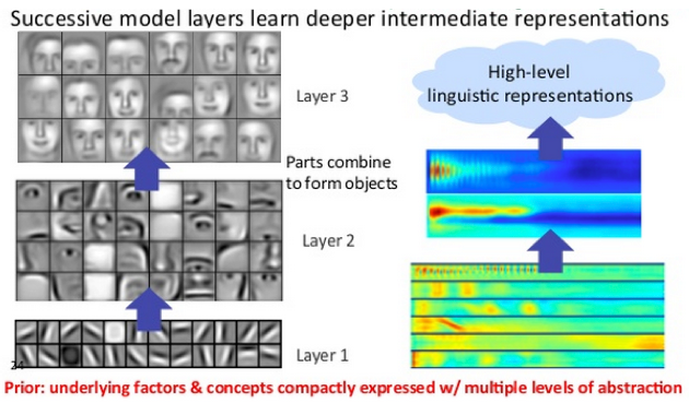
What the Network Learns to Do
The training objective specifies what counts as a useful result. A crop-yield model can minimize the difference between predicted and observed harvests. A classifier can minimize a loss based on the probability assigned to the correct category. An autoencoder compares a reconstruction with its input; a next-character model learns to predict a target drawn from the text itself.
Those objectives produce different learning signals. Reconstruction is one way to train a representation. Other methods learn from category labels or from relationships within the data. Hidden layers are trained according to how their computations contribute to the network’s objective.
The output layer must suit that objective. Here are common choices:
| Task | Output | Example loss |
|---|---|---|
| Predict a continuous quantity | A value from a linear output layer | Squared error |
| Predict one of two categories | A sigmoid probability | Binary cross-entropy |
| Predict one of several mutually exclusive categories | A softmax probability distribution | Categorical cross-entropy |
Learning features reduces the need to specify every useful pattern by hand. It still requires choosing an objective and suitable data, then evaluating the model on examples withheld from training.
Example: Feedforward Networks
A feedforward network computes its prediction by passing an input through successive layers. During training, we compare that prediction with a target and calculate a loss, a number that measures the mismatch. Backpropagation calculates how the loss changes with each parameter; an optimizer uses those derivatives to update the parameters.
We can follow the forward calculation before considering an update. The crop example begins with a familiar statistical model, then adds hidden layers.
Multiple Linear Regression
A linear regression with one input has the form y_hat = w*x + b. For a crop, x might be fertilizer applied and y_hat the predicted yield. The coefficient w determines how the prediction changes as fertilizer increases, while the bias b sets its value when x is zero.
Adding sunlight and rainfall gives a multiple linear regression:
y_hat = w_f*fertilizer + w_s*sunlight + w_r*rainfall + b
This model gives each input a fixed coefficient. A dense neural-network layer performs a weighted sum and adds a bias at each unit, then applies an activation function to the result. The Keras Dense-layer reference describes this operation. A hidden unit’s output becomes an input to the next layer.
Why Add an Activation Function?
Stacking weighted sums and biases without nonlinear activations still gives one affine transformation, a weighted sum with an offset. For two layers, expanding W2*(W1*x + b1) + b2 gives (W2*W1)*x + (W2*b1 + b2). The two stages collapse into one.
A nonlinear activation lets successive layers represent relationships that a single affine transformation cannot. Activations transform numerical values, and their output ranges depend on the function. The Keras activation reference defines these functions:
| Activation | Operation | Output range |
|---|---|---|
| ReLU | max(z, 0) |
Zero and positive values, with no upper limit |
| Sigmoid | 1 / (1 + exp(-z)) |
Between 0 and 1 |
| Tanh | Hyperbolic tangent of z |
Between -1 and 1 |
| Hard tanh | Clip z below -1 or above 1 |
From -1 to 1, including the endpoints |
For example, ReLU maps -2 to 0 and leaves 3 as 3. We will use it after each hidden layer. The output layer will leave its weighted sum unchanged so that the network produces a continuous yield estimate.
Crop Yield Through Two Hidden Layers
Suppose fertilizer, sunlight and rainfall have been rescaled into numerical features, in that order. Our example input is x = [2, 1, 3]. These feature values are dimensionless; the output is a yield in tonnes per hectare.
We will choose the weights and biases by hand to make the arithmetic visible. They illustrate a network calculation and have not been fitted to agricultural data. The network has three input features, two units in each of two hidden layers, and one output:
3 inputs → 2 hidden units → 2 hidden units → 1 yield prediction
Treat x as a column vector with shape (3, 1). A row in each weight matrix supplies the weights for one unit. The biases and hidden activations are also column vectors; compact lists below show their entries.
W1 = [[ 1, 0, 1],     shape: (2, 3)
      [-1, 1, 0]]
b1 = [-1, 0]          shape: (2, 1)

W2 = [[0.5,  1],      shape: (2, 2)
      [  1, -1]]
b2 = [-1, -2]         shape: (2, 1)

W3 = [[2, 1.5]]       shape: (1, 2)
b3 = 1                one output bias
The first hidden layer computes two weighted sums. Component indices start at zero, as in the Python code below:
z1[0] =  1*2 + 0*1 + 1*3 - 1 =  4
z1[1] = -1*2 + 1*1 + 0*3 + 0 = -1
h1 = ReLU(z1) = [4, 0]           shape: (2, 1)
The second hidden layer receives [4, 0]:
z2[0] = 0.5*4 + 1*0 - 1 = 1
z2[1] =   1*4 - 1*0 - 2 = 2
h2 = ReLU(z2) = [1, 2]      shape: (2, 1)
The output layer combines those two values:
y_hat = 2*1 + 1.5*2 + 1 = 6 tonnes per hectare
The chosen weights suppress the first layer’s second unit for this input. A different input can change which ReLU units pass a positive value.
This Python code reproduces the calculation using only the standard library. It stores vectors as flat lists and weight matrices as lists of rows.
def dense(inputs, weights, biases):
    return [sum(w * x for w, x in zip(row, inputs)) + bias
            for row, bias in zip(weights, biases)]


def relu(values):
    return [max(0.0, value) for value in values]


x = [2.0, 1.0, 3.0]
z1 = dense(x, [[1, 0, 1], [-1, 1, 0]], [-1, 0])
h1 = relu(z1)
z2 = dense(h1, [[0.5, 1], [1, -1]], [-1, -2])
h2 = relu(z2)
y_hat = dense(h2, [[2, 1.5]], [1])[0]

print("First layer:", z1, "->", h1)
print("Second layer:", z2, "->", h2)
print("Predicted yield:", y_hat, "tonnes per hectare")
Gradient Descent
Suppose the observed yield for this example was 5 tonnes per hectare. The prediction is too high by 1, and its squared-error loss is (6 - 5)^2 = 1. The gradient tells us how that loss would change if we changed a parameter slightly.
For the output weight multiplying the first component of h2, call it w, the derivative is:
dLoss/dw = 2*(y_hat - y)*h2[0] = 2*(6 - 5)*1 = 2
A gradient-descent step with learning rate 0.1 subtracts 0.1*2 from that weight, changing it from 2 to 1.8. Holding the other parameters fixed, the prediction becomes 1.8*1 + 1.5*2 + 1 = 5.8, and the loss falls to 0.64.
In ordinary training, backpropagation uses the chain rule to calculate gradients for parameters throughout the network. An optimizer updates the trainable parameters using losses over a batch of examples, then repeats the forward calculation. We use validation data to choose settings and decide when to stop, and reserve test data to evaluate predictions on new harvests.
Logistic Regression and Classification Outputs
The crop model ends in a continuous prediction. For binary classification, we can instead apply a sigmoid to the output score z, giving p = 1 / (1 + exp(-z)). The score includes a weighted sum of features and a bias. As it rises, the estimated probability of the positive class approaches 1; as it falls, that probability approaches 0.
A probability and a class decision are separate quantities. A model might estimate a 0.8 probability that an email is spam. A threshold of 0.5 would classify it as spam; changing the threshold changes which emails get flagged. Choose that threshold on validation data with the cost of false alarms and missed spam in mind. The logistic regression guide develops this calculation.
For several mutually exclusive categories, such as digit labels from 0 to 9, a softmax output gives probabilities that sum to 1. For labels that can apply simultaneously, a model can use a separate sigmoid for each label. The task determines the output and loss, while the hidden layers learn representations that help make that prediction.
Neural Networks & Artificial Intelligence
In some circles, neural networks are synonymous with AI. In others, they are thought of as a “brute force” technique, characterized by a lack of intelligence, because they start with a blank slate, and they hammer their way through to an accurate model. By this interpretation,neural networks are effective, but inefficient in their approach to modeling, since they don’t make assumptions about functional dependencies between output and input.
For what it’s worth, the foremost AI research groups are pushing the edge of the discipline by training larger and larger neural networks. Brute force works. It is a necessary, if not sufficient, condition to AI breakthroughs. OpenAI’s pursuit of more general AI emphasizes a brute force approach, which has proven effective with well-known models such as GPT-3.
Algorithms such as Hinton’s capsule networks require far fewer instances of data to converge on an accurate model; that is, present research has the potential to resolve the brute force inefficiencies of deep learning.
While neural networks are useful as a function approximator, mapping inputs to outputs in many tasks of perception, to achieve a more general intelligence, they can be combined with other AI methods to perform more complex tasks. For example, deep reinforcement learning embeds neural networks within a reinforcement learning framework, where they map actions to rewards in order to achieve goals. Deepmind’s victories in video games and the board game of go are good examples.
Further Reading
- Reinforcement Learning and Neural Networks
- Recurrent Neural Networks (RNNs) and LSTMs
- Word2vec and Neural Word Embeddings
- Convolutional Neural Networks (CNNs) and Image Processing
- Accuracy, Precision and Recall
- Attention Mechanisms and Transformers
- Eigenvectors, Eigenvalues, PCA, Covariance and Entropy
- Graph Analytics and Deep Learning
- Symbolic Reasoning and Machine Learning
- Markov Chain Monte Carlo, AI and Markov Blankets
- Generative Adversarial Networks (GANs)
- AI vs Machine Learning vs Deep Learning
- Multilayer Perceptrons (MLPs)
- Simulations, Optimization and AI
- A Recipe for Training Neural Networks, by Andrej Karpathy