Contents
- Feedforward Networks
- Recurrent Networks
- A Worked Recurrent Network
- Inputs, Targets and Prediction Error
- Backpropagation Through Time
- Vanishing and Exploding Gradients
- Long Short-Term Memory Units (LSTMs)
- Capturing Diverse Time Scales
- Gated Recurrent Units (GRUs)
- LSTM Hyperparameter Tuning
- Resources
Introduction
A recurrent neural network (RNN) processes a sequence by carrying information from one step to the next. That information gives the current input a context: an earlier word can change how a later word is interpreted, and earlier sensor readings can help predict the next reading.
Long short-term memory networks, or LSTMs, are RNNs with gates that control what their memory retains and exposes. We will first follow a small recurrent network through two characters, then examine how an LSTM changes the memory mechanism.
Review of Feedforward Networks
A feedforward network transforms its input through a succession of layers. An image classifier, for example, turns the pixels of a photograph into scores for categories such as cat or elephant. A regression network can instead produce a continuous quantity, such as tomorrow’s temperature.
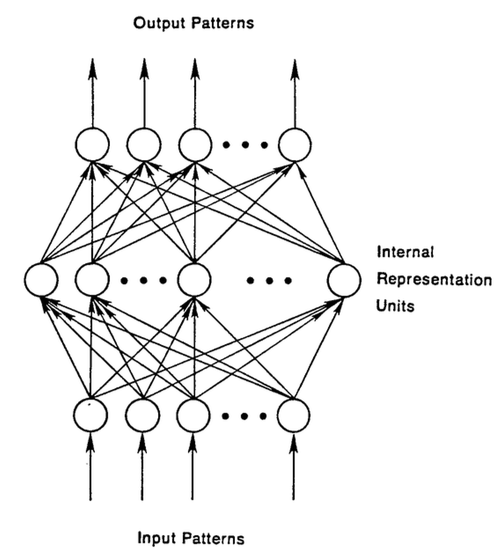
An ordinary feedforward network processes each supplied example without carrying a hidden state over from the previous example. We can give it a fixed window of past observations as part of its input. A recurrent network builds that connection into its computation: it updates a state as each observation arrives.
Recurrent Neural Networks
Imagine hearing the sounds “Hi Jack!” near Jack’s house and then hearing them on an airplane. The preceding situation changes the interpretation. A recurrent network carries its own numerical context, called a hidden state, through the sequence it is processing.
At each step, the network combines the current input with its previous hidden state to compute a new hidden state. A separate output layer can use that state to predict the next character or classify the sequence. The state can carry information that is useful later even when the current prediction does not expose it.
The network’s weights and state change on different schedules. Training adjusts the weights across examples. During ordinary prediction, those weights stay fixed while the hidden state changes with each new input. We normally reset the state at the boundary between independent sequences; we can carry it forward when a sequence continues in another chunk.
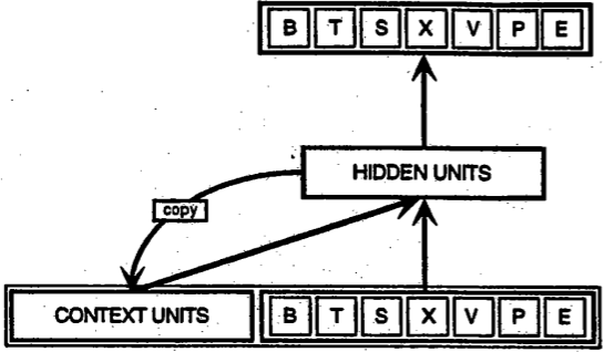
In this Elman network diagram, the context units carry the previous hidden activations. For a simple recurrent layer, we can write the update as:
h_t = tanh(W_x x_t + W_h h_(t-1) + b_h)
Here x_t is the current input vector and h_(t-1) is the previous hidden state. The matrices W_x and W_h weight their contributions; b_h is a learned offset. The same parameters are used at every step. The nonlinear function tanh maps each resulting value between -1 and 1. The PyTorch RNN documentation gives this recurrence and its input conventions.
For next-character prediction, an output layer turns h_t into one score per possible next character. Softmax converts those scores into probabilities:
z_t = W_y h_t + b_y
p_t[j] = exp(z_t[j]) / sum_k exp(z_t[k])
The hidden state h_t and the prediction p_t have different jobs and can have different sizes. A recurrent model can make a prediction at every step, or use its final state to make one prediction about the whole sequence.
Following Two Characters Through a Recurrent State
Take a vocabulary of three symbols, [a, b, <end>], where <end> marks the end of a sequence. A one-hot encoding gives each symbol its own position: a = [1, 0, 0], b = [0, 1, 0], and <end> = [0, 0, 1].
Our demonstration network has one hidden value, starts at h_0 = 0, and uses these hand-chosen weights:
W_x = [[1, 0, 0]]  shape: (1, 3)
W_h = [[0.5]]      shape: (1, 1)
b_h = 0
The input contributes 1 for a and 0 for either other symbol. At every step, we add half the previous state and apply tanh.
| Sequence | State after the first character | State after the second character |
|---|---|---|
ab |
tanh(1 + 0.5 × 0) = 0.761594 |
tanh(0 + 0.5 × 0.761594) = 0.363399 |
ba |
tanh(0 + 0.5 × 0) = 0 |
tanh(1 + 0.5 × 0) = 0.761594 |
Both sequences contain the same characters. Their final states differ because the first state changes the calculation at the second step. The weights stay the same throughout both runs.
Inputs, Targets and Prediction Error
To train on the sequence ab<end>, shift the targets one position ahead of the inputs:
| Step | Input | Target: the next symbol |
|---|---|---|
| 1 | a |
b |
| 2 | b |
<end> |
These targets come from the sequence itself. Next-character prediction has a target at each step even though a person does not have to annotate the text with separate labels.
For this example, use the axis order batch, time, features. One two-step sequence with three input features has shape (1, 2, 3). Its hidden states have shape (1, 2, 1). The output probabilities and one-hot targets each have shape (1, 2, 3); batched integer targets [[1, 2]], using the vocabulary’s zero-based indices, instead have shape (1, 2). Libraries differ in their default axis order, so check the API when loading data.
Choose an output matrix W_y = [[-1], [1], [0]], with shape (3, 1), and zero output biases. Its scores are [-h_t, h_t, 0]. After reading a, the state is 0.761594, and softmax assigns probabilities of approximately 0.129391 to a, 0.593494 to b, and 0.277115 to <end>.
The target is b. Its cross-entropy loss is -log(p(b)), using the natural logarithm, or about 0.522. The most probable symbol is correct, but the loss still measures how much probability the model assigned to that target. At the second step, the target is <end>; the same output weights favor b, so the model makes a wrong prediction. Training uses the losses across the sequence.
This Python example reproduces the states and predictions using only the standard library. Its weights are chosen to expose the calculation; it does not train a language model.
from math import exp, log, tanh

vocab = ("a", "b", "<end>")
input_weight = {"a": 1.0, "b": 0.0, "<end>": 0.0}


def hidden_states(sequence):
    h = 0.0
    states = []
    for symbol in sequence:
        h = tanh(input_weight[symbol] + 0.5 * h)
        states.append(h)
    return states


def probabilities(h):
    scores = (-h, h, 0.0)
    largest = max(scores)
    values = [exp(score - largest) for score in scores]
    return [value / sum(values) for value in values]


for sequence in ("ab", "ba"):
    print(sequence, [round(h, 6) for h in hidden_states(sequence)])

for symbol, target, h in zip(("a", "b"), ("b", "<end>"),
                             hidden_states("ab")):
    p = probabilities(h)
    loss = -log(p[vocab.index(target)])
    prediction = vocab[max(range(len(p)), key=p.__getitem__)]
    print(symbol, "target:", target, "prediction:", prediction,
          "probabilities:", [round(value, 6) for value in p],
          "loss:", round(loss, 6))
Backpropagation Through Time (BPTT)
Training uses the prediction loss to calculate how each parameter contributed to the error. For softmax followed by cross-entropy, the derivative with respect to each output score is its predicted probability minus its target indicator, which is 1 for the correct symbol and 0 for the others.
Considering the first step’s loss alone, the derivative for b’s score is approximately 0.593494 - 1 = -0.406506. A gradient-descent update subtracts the derivative times a learning rate, so this contribution pushes b’s output bias upward. The derivatives for the other two scores are positive, pushing their biases down. The output weights also receive gradients through their connection to the hidden state. Training on the whole sequence combines these contributions with those from the second step.
The loss at the second step depends on h_2, which depends on h_1. Backpropagation through time follows those connections backward using the chain rule. Because the recurrent weights are shared across steps, their gradient accumulates contributions from each use. An optimizer then updates the weights and biases. Those updated parameters govern the next forward pass.
Truncated BPTT
Long sequences can require too much memory to retain every intermediate calculation for a backward pass. Truncated BPTT limits that pass to a shorter window. A model can carry its hidden state into the next window while detaching it from the earlier computation, so information can continue forward even though gradients stop at the boundary. That limits how far a later loss can directly train an earlier computation. Ilya Sutskever’s dissertation discusses training recurrent networks.
Vanishing and Exploding Gradients
When training follows a recurrent state backward through many steps, it repeatedly multiplies derivatives. Products of small factors can shrink toward zero, leaving an early input with very little influence on the weight update. Large factors can make the gradients grow enough to destabilize training. These are the vanishing and exploding gradient problems.
Our one-value network makes the shrinking visible. The derivative of the new state with respect to the previous state is 0.5 × (1 - h_t²), whose magnitude is at most 0.5. Across ten steps, the product along that recurrent path is at most 0.5^10, about 0.00098. The state can still carry information forward while the training signal reaching earlier steps becomes small.
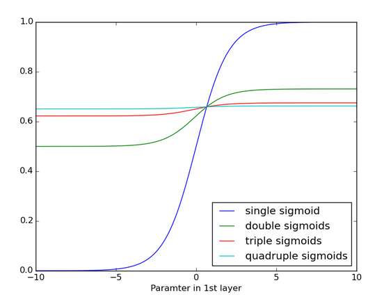
Gradient clipping limits the size of an update’s gradient and can help with exploding gradients. It does not restore a gradient that has already vanished. LSTMs change the recurrent computation to provide a more direct path for retaining state and passing gradients through time.
Long Short-Term Memory Units (LSTMs)
Sepp Hochreiter and Jürgen Schmidhuber introduced LSTM in their 1997 paper. The commonly used version described here includes a forget gate, added in later work.
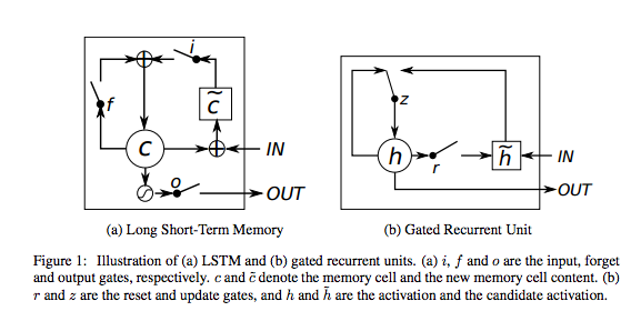
An LSTM carries a cell state, c_t, alongside its hidden state, h_t. The cell state holds information that can persist across steps. The hidden state exposes a gated transformation of that information to the next layer or an output predictor, and also helps compute the next step’s gates.
A gate produces a vector of values between 0 and 1. Multiplying a signal by a gate scales each component separately: a value near 0 largely suppresses it, while a value near 1 largely preserves it. The gates can be partly open.
| Gate | What it controls |
|---|---|
Forget gate f_t |
How much of the previous cell state to retain |
Input gate i_t |
How much of the proposed new content to write |
Output gate o_t |
How much of the transformed cell state to expose as the hidden state |
In the LSTM variant below, each gate uses the current input x_t and previous hidden state h_(t-1). Each has its own learned weights and bias. The candidate content g_t uses the same inputs with a tanh activation. Here sigmoid produces values between 0 and 1, and * means element-by-element multiplication:
f_t = sigmoid(W_f x_t + U_f h_(t-1) + b_f)
i_t = sigmoid(W_i x_t + U_i h_(t-1) + b_i)
o_t = sigmoid(W_o x_t + U_o h_(t-1) + b_o)
g_t = tanh(W_g x_t + U_g h_(t-1) + b_g)

c_t = f_t * c_(t-1) + i_t * g_t
h_t = o_t * tanh(c_t)
These are the state updates documented in the PyTorch LSTM reference. The forget gate is computed with a sigmoid. When it is close to 1, multiplication carries almost all of the previous cell state forward.
For one component, suppose the previous cell state is 0.8, the forget gate is 0.9, the input gate is 0.2, and the candidate content is -0.5. The new cell state is:
c_t = 0.9 × 0.8 + 0.2 × (-0.5) = 0.62
If the output gate is 0.5, the corresponding hidden value is 0.5 × tanh(0.62), approximately 0.276. The cell retains 0.62 while exposing 0.276. Closing the output gate would suppress that exposure without itself erasing the cell state.
The addition in the cell update gives retained information a direct path to the next step. Holding the gate values fixed, the derivative along that path is f_t. When forget gates remain near 1, this path can carry gradients across many steps with less shrinkage. Other paths also contribute to the full gradient; an LSTM’s ability to learn a long dependency still depends on training and the data.
Resetting states between unrelated documents is a separate choice made by the program running the model. Within a document, the learned gates control how much context to retain as the sequence unfolds.
Capturing Diverse Time Scales and Remote Dependencies
You may also wonder what the precise value is of input gates that protect a memory cell from new data coming in, and output gates that prevent it from affecting certain outputs of the RNN. You can think of LSTMs as allowing a neural network to operate on different scales of time at once.
Let’s take a human life, and imagine that we are receiving various streams of data about that life in a time series. Geolocation at each time step is pretty important for the next time step, so that scale of time is always open to the latest information.
Perhaps this human is a diligent citizen who votes every couple years. On democratic time, we would want to pay special attention to what they do around elections, before they return to making a living, and away from larger issues. We would not want to let the constant noise of geolocation affect our political analysis.
If this human is also a diligent daughter, then maybe we can construct a familial time that learns patterns in phone calls which take place regularly every Sunday and spike annually around the holidays. Little to do with political cycles or geolocation.
Other data is like that. Music is polyrhythmic. Text contains recurrent themes at varying intervals. Stock markets and economies experience jitters within longer waves. They operate simultaneously on different time scales that LSTMs can capture.
Gated Recurrent Units (GRUs)
A gated recurrent unit (GRU) keeps a single hidden state. Its update gate controls the mixture of retained state and candidate content, while its reset gate controls how the previous state contributes to the candidate. A standard GRU has no separate cell state or output gate. The comparison by Chung and colleagues describes both architectures and evaluates them on sequence-modeling tasks.
LSTM Hyperparameter Tuning
Watch out for overfitting: training performance can keep improving while predictions on new data get worse. Regularization, such as weight penalties or dropout, can help. Compare simpler and larger networks on validation data to learn whether extra capacity helps your task.
Use a validation set to choose hyperparameters and monitor early stopping across epochs (complete passes through the training data). Reserve a separate test set for the final evaluation. Using test results to decide when to stop leaks information into model selection. For forecasting, preserve time order so that evaluation measures predictions of later observations. See the scikit-learn guide to validation and time-series splits.
Treat the learning rate and optimizer as choices to compare on validation data. The same applies to adding layers or changing an activation function. Fit normalization on training data, then apply that transformation to the held-out sets. For a regression task, mean squared error with a linear output is one starting point; choose the loss and output activation to suit the quantity you want to predict.
Resources
- DRAW: A Recurrent Neural Network For Image Generation; (attention models)
- Gated Feedback Recurrent Neural Networks
- Recurrent Neural Networks; Juergen Schmidhuber
- Modeling Sequences With RNNs and LSTMs; Geoff Hinton
- The Unreasonable Effectiveness of Recurrent Neural Networks; Andrej Karpathy
- Understanding LSTMs; Christopher Olah
- Backpropagation Through Time: What It Does and How to Do It; Paul Werbos
- Empirical Evaluation of Gated Recurrent Neural Networks on Sequence Modeling; Cho et al
- Training Recurrent Neural Networks; Ilya Sutskever’s Dissertation
- Supervised Sequence Labelling with Recurrent Neural Networks; Alex Graves
- Long Short-Term Memory in Recurrent Neural Networks; Felix Gers
- LSTM: A Search Space Oddyssey; Klaus Greff et al
Other Pathmind Wiki Posts
- Neural Networks and Deep Learning
- Word2vec and Neural Word Embeddings
- Convolutional Neural Networks (CNNs) and Image Processing
- Accuracy, Precision and Recall
- Attention Mechanisms and Transformers
- Eigenvectors, Eigenvalues, PCA, Covariance and Entropy
- Graph Analytics and Deep Learning
- Symbolic Reasoning and Machine Learning
- Markov Chain Monte Carlo, AI and Markov Blankets
- Deep Reinforcement Learning
- Generative Adversarial Networks (GANs)
- AI vs Machine Learning vs Deep Learning
- Multilayer Perceptrons (MLPs)