A Beginner's Guide to Convolutional Neural Networks (CNNs)
Contents
- Introduction to Convolutional Neural Networks
- Images Are 4-D Tensors?
- Definition of Convolutional Nets
- How Convolutional Nets Work
- Maxpooling/Downsampling
- Just Show Me the Code
- More ConvNet Resources
Introduction to Deep Convolutional Neural Networks
Convolutional neural networks are neural networks used primarily to classify images (i.e. name what they see), cluster images by similarity (photo search), and perform object recognition within scenes. For example, convolutional neural networks (ConvNets or CNNs) are used to identify faces, individuals, street signs, tumors, platypuses (platypi?) and many other aspects of visual data.
The efficacy of convolutional nets in image recognition is one of the main reasons why the world has woken up to the efficacy of deep learning. In a sense, CNNs are the reason why deep learning is famous. The success of a deep convolutional architecture called AlexNet in the 2012 ImageNet competition was the shot heard round the world. CNNs are powering major advances in computer vision (CV), which has obvious applications for self-driving cars, robotics, drones, security, medical diagnoses, and treatments for the visually impaired.
Convolutional networks can also perform more banal (and more profitable), business-oriented tasks such as optical character recognition (OCR) to digitize text and make natural-language processing possible on analog and hand-written documents, where the images are symbols to be transcribed.
CNNs are not limited to image recognition, however. They have been applied directly to text analytics. And they be applied to sound when it is represented visually as a spectrogram, and graph data with graph convolutional networks.
Learn How to Apply AI to Simulations »
Images Are 4-D Tensors?
Convolutional neural networks ingest and process images as tensors, and tensors are matrices of numbers with additional dimensions.
They can be hard to visualize, so let’s approach them by analogy. A scalar is just a number, such as 7; a vector is a list of numbers (e.g., [7,8,9]); and a matrix is a rectangular grid of numbers occupying several rows and columns like a spreadsheet. Geometrically, if a scalar is a zero-dimensional point, then a vector is a one-dimensional line, a matrix is a two-dimensional plane, a stack of matrices is a three-dimensional cube, and when each element of those matrices has a stack of feature maps attached to it, you enter the fourth dimension. For reference, here’s a 2 x 2 matrix:
[ 1, 2 ]
[ 5, 8 ]
A tensor encompasses the dimensions beyond that 2-D plane. You can easily picture a three-dimensional tensor, with the array of numbers arranged in a cube. Here’s a 2 x 3 x 2 tensor presented flatly (picture the bottom element of each 2-element array extending along the z-axis to intuitively grasp why it’s called a 3-dimensional array):
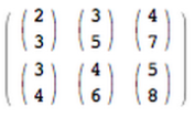
In code, the tensor above would appear like this: [[[2,3],[3,5],[4,7]],[[3,4],[4,6],[5,8]]]. And here’s a visual:
In other words, tensors are formed by arrays nested within arrays, and that nesting can go on infinitely, accounting for an arbitrary number of dimensions far greater than what we can visualize spatially. A 4-D tensor would simply replace each of these scalars with an array nested one level deeper. Convolutional networks deal in 4-D tensors like the one below (notice the nested array).
With some tools, you will see NDArray used synonymously with tensor, or multi-dimensional array. A tensor’s dimensionality (1,2,3…n) is called its order; i.e. a fifth-order tensor would have five dimensions.
The width and height of an image are easily understood. The depth is necessary because of how colors are encoded. Red-Green-Blue (RGB) encoding, for example, produces an image three layers deep. Each layer is called a “channel”, and through convolution it produces a stack of feature maps (explained below), which exist in the fourth dimension, just down the street from time itself. (Features are just details of images, like a line or curve, that convolutional networks create maps of.)
So instead of thinking of images as two-dimensional areas, in convolutional nets they are treated as four-dimensional volumes. These ideas will be explored more thoroughly below.
Convolutional Definition
From the Latin convolvere, “to convolve” means to roll together. For mathematical purposes, a convolution is the integral measuring how much two functions overlap as one passes over the other. Think of a convolution as a way of mixing two functions by multiplying them.
Credit: Mathworld. “The green curve shows the convolution of the blue and red curves as a function of t, the position indicated by the vertical green line. The gray region indicates the product g(tau)f(t-tau) as a function of t, so its area as a function of t is precisely the convolution.”
Look at the tall, narrow bell curve standing in the middle of a graph. The integral is the area under that curve. Near it is a second bell curve that is shorter and wider, drifting slowly from the left side of the graph to the right. The product of those two functions’ overlap at each point along the x-axis is their convolution. So in a sense, the two functions are being “rolled together.”
With image analysis, the static, underlying function (the equivalent of the immobile bell curve) is the input image being analyzed, and the second, mobile function is known as the filter, because it picks up a signal or feature in the image. The two functions relate through multiplication. To visualize convolutions as matrices rather than as bell curves, please see Andrej Karpathy’s excellent animation under the heading “Convolution Demo.”
The next thing to understand about convolutional nets is that they are passing many filters over a single image, each one picking up a different signal. At a fairly early layer, you could imagine them as passing a horizontal line filter, a vertical line filter, and a diagonal line filter to create a map of the edges in the image.
Convolutional networks take those filters, slices of the image’s feature space, and map them one by one; that is, they create a map of each place that feature occurs. By learning different portions of a feature space, convolutional nets allow for easily scalable and robust feature engineering.
(Note that convolutional nets analyze images differently than RBMs. While RBMs learn to reconstruct and identify the features of each image as a whole, convolutional nets learn images in pieces that we call feature maps.)
So convolutional networks perform a sort of search. Picture a small magnifying glass sliding left to right across a larger image, and recommencing at the left once it reaches the end of one pass (like typewriters do). That moving window is capable recognizing only one thing, say, a short vertical line. Three dark pixels stacked atop one another. It moves that vertical-line-recognizing filter over the actual pixels of the image, looking for matches.
Each time a match is found, it is mapped onto a feature space particular to that visual element. In that space, the location of each vertical line match is recorded, a bit like birdwatchers leave pins in a map to mark where they last saw a great blue heron. A convolutional net runs many, many searches over a single image – horizontal lines, diagonal ones, as many as there are visual elements to be sought.
Convolutional nets perform more operations on input than just convolutions themselves.
After a convolutional layer, input is passed through a nonlinear transform such as tanh or rectified linear unit, which will squash input values into a range between -1 and 1.
How Convolutional Neural Networks Work
The first thing to know about convolutional networks is that they don’t perceive images like humans do. Therefore, you are going to have to think in a different way about what an image means as it is fed to and processed by a convolutional network.
Convolutional networks perceive images as volumes; i.e. three-dimensional objects, rather than flat canvases to be measured only by width and height. That’s because digital color images have a red-blue-green (RGB) encoding, mixing those three colors to produce the color spectrum humans perceive. A convolutional network ingests such images as three separate strata of color stacked one on top of the other.
So a convolutional network receives a normal color image as a rectangular box whose width and height are measured by the number of pixels along those dimensions, and whose depth is three layers deep, one for each letter in RGB. Those depth layers are referred to as channels.
As images move through a convolutional network, we will describe them in terms of input and output volumes, expressing them mathematically as matrices of multiple dimensions in this form: 30x30x3. From layer to layer, their dimensions change for reasons that will be explained below.
You will need to pay close attention to the precise measures of each dimension of the image volume, because they are the foundation of the linear algebra operations used to process images.
Now, for each pixel of an image, the intensity of R, G and B will be expressed by a number, and that number will be an element in one of the three, stacked two-dimensional matrices, which together form the image volume.
Those numbers are the initial, raw, sensory features being fed into the convolutional network, and the ConvNets purpose is to find which of those numbers are significant signals that actually help it classify images more accurately. (Just like other feedforward networks we have discussed.)
Rather than focus on one pixel at a time, a convolutional net takes in square patches of pixels and passes them through a filter. That filter is also a square matrix smaller than the image itself, and equal in size to the patch. It is also called a kernel, which will ring a bell for those familiar with support-vector machines, and the job of the filter is to find patterns in the pixels.
Credit for this excellent animation goes to Andrej Karpathy.
Imagine two matrices. One is 30x30, and another is 3x3. That is, the filter covers one-hundredth of one image channel’s surface area.
We are going to take the dot product of the filter with this patch of the image channel. If the two matrices have high values in the same positions, the dot product’s output will be high. If they don’t, it will be low. In this way, a single value – the output of the dot product – can tell us whether the pixel pattern in the underlying image matches the pixel pattern expressed by our filter.
Let’s imagine that our filter expresses a horizontal line, with high values along its second row and low values in the first and third rows. Now picture that we start in the upper lefthand corner of the underlying image, and we move the filter across the image step by step until it reaches the upper righthand corner. The size of the step is known as stride. You can move the filter to the right one column at a time, or you can choose to make larger steps.
At each step, you take another dot product, and you place the results of that dot product in a third matrix known as an activation map. The width, or number of columns, of the activation map is equal to the number of steps the filter takes to traverse the underlying image. Since larger strides lead to fewer steps, a big stride will produce a smaller activation map. This is important, because the size of the matrices that convolutional networks process and produce at each layer is directly proportional to how computationally expensive they are and how much time they take to train. A larger stride means less time and compute.
A filter superimposed on the first three rows will slide across them and then begin again with rows 4-6 of the same image. If it has a stride of three, then it will produce a matrix of dot products that is 10x10. That same filter representing a horizontal line can be applied to all three channels of the underlying image, R, G and B. And the three 10x10 activation maps can be added together, so that the aggregate activation map for a horizontal line on all three channels of the underlying image is also 10x10.
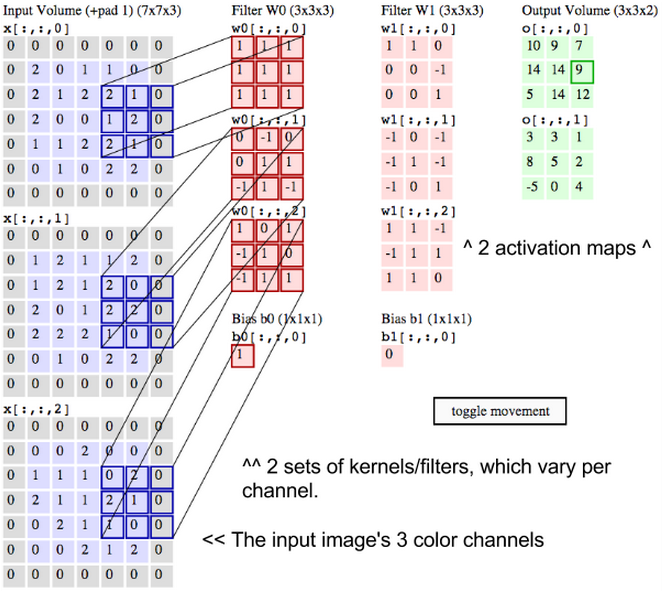
Now, because images have lines going in many directions, and contain many different kinds of shapes and pixel patterns, you will want to slide other filters across the underlying image in search of those patterns. You could, for example, look for 96 different patterns in the pixels. Those 96 patterns will create a stack of 96 activation maps, resulting in a new volume that is 10x10x96. In the diagram below, we’ve relabeled the input image, the kernels and the output activation maps to make sure we’re clear.
What we just described is a convolution. You can think of Convolution as a fancy kind of multiplication used in signal processing. Another way to think about the two matrices creating a dot product is as two functions. The image is the underlying function, and the filter is the function you roll over it.
One of the main problems with images is that they are high-dimensional, which means they cost a lot of time and computing power to process. Convolutional networks are designed to reduce the dimensionality of images in a variety of ways. Filter stride is one way to reduce dimensionality. Another way is through downsampling.
Max Pooling/Downsampling with CNNs
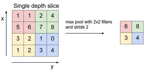
The next layer in a convolutional network has three names: max pooling, downsampling and subsampling. The activation maps are fed into a downsampling layer, and like convolutions, this method is applied one patch at a time. In this case, max pooling simply takes the largest value from one patch of an image, places it in a new matrix next to the max values from other patches, and discards the rest of the information contained in the activation maps.
 Credit to Andrej Karpathy.
Only the locations on the image that showed the strongest correlation to each feature (the maximum value) are preserved, and those maximum values combine to form a lower-dimensional space.
Much information about lesser values is lost in this step, which has spurred research into alternative methods. But downsampling has the advantage, precisely because information is lost, of decreasing the amount of storage and processing required.
Alternating Layers
The image below is another attempt to show the sequence of transformations involved in a typical convolutional network.
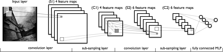
From left to right you see:
- The actual input image that is scanned for features. The light rectangle is the filter that passes over it.
- Activation maps stacked atop one another, one for each filter you employ. The larger rectangle is one patch to be downsampled.
- The activation maps condensed through downsampling.
- A new set of activation maps created by passing filters over the first downsampled stack.
- The second downsampling, which condenses the second set of activation maps.
- A fully connected layer that classifies output with one label per node.
As more and more information is lost, the patterns processed by the convolutional net become more abstract and grow more distant from visual patterns we recognize as humans. So forgive yourself, and us, if convolutional networks do not offer easy intuitions as they grow deeper.
Further Reading
- Deep Neural Networks
- Recurrent Neural Networks (RNNs) and LSTMs
- Word2vec and Neural Word Embeddings
- Accuracy, Precision and Recall
- Attention Mechanisms and Transformers
- Eigenvectors, Eigenvalues, PCA, Covariance and Entropy
- Graph Analytics and Deep Learning
- Symbolic Reasoning and Machine Learning
- Markov Chain Monte Carlo, AI and Markov Blankets
- Deep Reinforcement Learning
- Generative Adversarial Networks (GANs)
- AI vs Machine Learning vs Deep Learning
- Multilayer Perceptrons (MLPs)

Chris V. Nicholson
Chris V. Nicholson is a venture partner at Page One Ventures. He previously led Pathmind and Skymind. In a prior life, Chris spent a decade reporting on tech and finance for The New York Times, Businessweek and Bloomberg, among others.