A Beginner's Guide to Eigenvectors, Eigenvalues, PCA, Covariance and Entropy

Contents

• Linear Transformations
• Principal Component Analysis (PCA)
• Covariance Matrix
• Change of Basis
• Entropy & Information Gain
• Just Give Me the Code
• Resources

This post introduces eigenvectors and their relationship to matrices in plain language and without a great deal of math. It builds on those ideas to explain covariance, principal component analysis, and information entropy.

The eigen in eigenvector comes from German, and it means something like “very own.” For example, in German, “mein eigenes Auto” means “my very own car.” So eigen denotes a special relationship between two things. Something particular, characteristic and definitive. This car, or this vector, is mine and not someone else’s.

Matrices, in linear algebra, are simply rectangular arrays of numbers, a collection of scalar values between brackets, like a spreadsheet. All square matrices (e.g. 2 x 2 or 3 x 3) have eigenvectors, and they have a very special relationship with them, a bit like Germans have with their cars.

Learn How to Apply AI to Simulations »

Linear Transformations

We’ll define that relationship after a brief detour into what matrices do, and how they relate to other numbers.

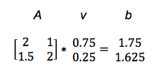
Matrices are useful because you can do things with them like add and multiply. If you multiply a vector v by a matrix A, you get another vector b, and you could say that the matrix performed a linear transformation on the input vector.

Av = b

It maps one vector v to another, b.

We’ll illustrate with a concrete example. (You can see how this type of matrix multiply, called a dot product, is performed here.)

So A turned v into b. In the graph below, we see how the matrix mapped the short, low line v, to the long, high one, b.

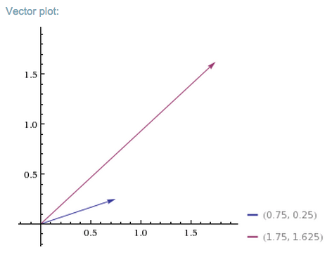
You could feed one positive vector after another into matrix A, and each would be projected onto a new space that stretches higher and farther to the right.

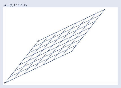
Imagine that all the input vectors v live in a normal grid, like this:

And the matrix projects them all into a new space like the one below, which holds the output vectors b:

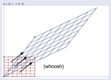
Here you can see the two spaces juxtaposed:

(Credit: William Gould, Stata Blog)

And here’s an animation that shows the matrix’s work transforming one space to another:

The blue lines are eigenvectors.

You can imagine a matrix like a gust of wind, an invisible force that produces a visible result. And a gust of wind must blow in a certain direction. The eigenvector tells you the direction the matrix is blowing in.

(Credit: Wikipedia)

So out of all the vectors affected by a matrix blowing through one space, which one is the eigenvector? It’s the one that that changes length but not direction; that is, the eigenvector is already pointing in the same direction that the matrix is pushing all vectors toward. An eigenvector is like a weathervane. An eigenvane, as it were.

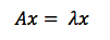
The definition of an eigenvector, therefore, is a vector that responds to a matrix as though that matrix were a scalar coefficient. In this equation, A is the matrix, x the vector, and lambda the scalar coefficient, a number like 5 or 37 or pi.

You might also say that eigenvectors are axes along which linear transformation acts, stretching or compressing input vectors. They are the lines of change that represent the action of the larger matrix, the very “line” in linear transformation.

Notice we’re using the plural – axes and lines. Just as a German may have a Volkswagen for grocery shopping, a Mercedes for business travel, and a Porsche for joy rides (each serving a distinct purpose), square matrices can have as many eigenvectors as they have dimensions; i.e. a 2 x 2 matrix could have two eigenvectors, a 3 x 3 matrix three, and an n x n matrix could have n eigenvectors, each one representing its line of action in one dimension.1

Because eigenvectors distill the axes of principal force that a matrix moves input along, they are useful in matrix decomposition; i.e. the diagonalization of a matrix along its eigenvectors. Because those eigenvectors are representative of the matrix, they perform the same task as the autoencoders employed by deep neural networks.

To quote Yoshua Bengio:

Many mathematical objects can be understood better by breaking them into constituent parts, or finding some properties of them that are universal, not caused by the way we choose to represent them.

For example, integers can be decomposed into prime factors. The way we represent the number 12 will change depending on whether we write it in base ten or in binary, but it will always be true that 12 = 2 × 2 × 3.

From this representation we can conclude useful properties, such as that 12 is not divisible by 5, or that any integer multiple of 12 will be divisible by 3.

Much as we can discover something about the true nature of an integer by decomposing it into prime factors, we can also decompose matrices in ways that show us information about their functional properties that is not obvious from the representation of the matrix as an array of elements.

One of the most widely used kinds of matrix decomposition is called eigen-decomposition, in which we decompose a matrix into a set of eigenvectors and eigenvalues.

Principal Component Analysis (PCA)

PCA is a tool for finding patterns in high-dimensional data such as images. Machine-learning practitioners sometimes use PCA to preprocess data for their neural networks. By centering, rotating and scaling data, PCA prioritizes dimensionality (allowing you to drop some low-variance dimensions) and can improve the neural network’s convergence speed and the overall quality of results.

To get to PCA, we’re going to quickly define some basic statistical ideas – mean, standard deviation, variance and covariance – so we can weave them together later. Their equations are closely related.

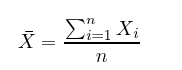
Mean is simply the average value of all x’s in the set X, which is found by dividing the sum of all data points by the number of data points, n.

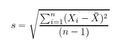
Standard deviation, as fun as that sounds, is simply the square root of the average square distance of data points to the mean. In the equation below, the numerator contains the sum of the differences between each datapoint and the mean, and the denominator is simply the number of data points (minus one), producing the average distance.

Variance is the measure of the data’s spread. If I take a team of Dutch basketball players and measure their height, those measurements won’t have a lot of variance. They’ll all be grouped above six feet.

But if I throw the Dutch basketball team into a classroom of psychotic kindergartners, then the combined group’s height measurements will have a lot of variance. Variance is the spread, or the amount of difference that data expresses.

Variance is simply standard deviation squared, and is often expressed as s^2.

For both variance and standard deviation, squaring the differences between data points and the mean makes them positive, so that values above and below the mean don’t cancel each other out.

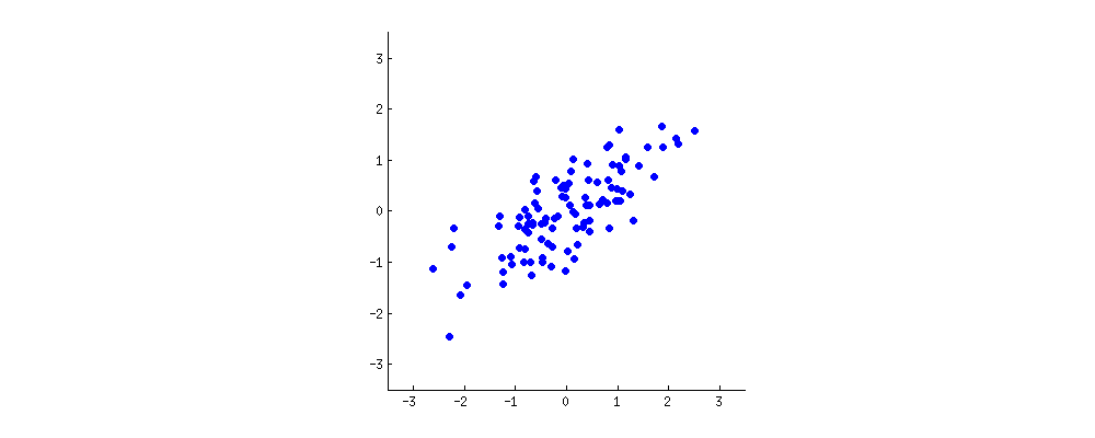
Let’s assume you plotted the age (x axis) and height (y axis) of those individuals (setting the mean to zero) and came up with an oblong scatterplot:

PCA attempts to draw straight, explanatory lines through data, like linear regression.

Each straight line represents a “principal component,” or a relationship between an independent and dependent variable. While there are as many principal components as there are dimensions in the data, PCA’s role is to prioritize them.

The first principal component bisects a scatterplot with a straight line in a way that explains the most variance; that is, it follows the longest dimension of the data. (This happens to coincide with the least error, as expressed by the red lines…) In the graph below, it slices down the length of the “baguette.”

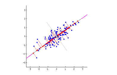
The second principal component cuts through the data perpendicular to the first, fitting the errors produced by the first. There are only two principal components in the graph above, but if it were three-dimensional, the third component would fit the errors from the first and second principal components, and so forth.

Covariance Matrix

While we introduced matrices as something that transformed one set of vectors into another, another way to think about them is as a description of data that captures the forces at work upon it, the forces by which two variables might relate to each other as expressed by their variance and covariance.

Imagine that we compose a square matrix of numbers that describe the variance of the data, and the covariance among variables. This is the covariance matrix. It is an empirical description of data we observe.

Finding the eigenvectors and eigenvalues of the covariance matrix is the equivalent of fitting those straight, principal-component lines to the variance of the data. Why? Because eigenvectors trace the principal lines of force, and the axes of greatest variance and covariance illustrate where the data is most susceptible to change.

Think of it like this: If a variable changes, it is being acted upon by a force known or unknown. If two variables change together, in all likelihood that is either because one is acting upon the other, or they are both subject to the same hidden and unnamed force.

When a matrix performs a linear transformation, eigenvectors trace the lines of force it applies to input; when a matrix is populated with the variance and covariance of the data, eigenvectors reflect the forces that have been applied to the given. One applies force and the other reflects it.

Eigenvalues are simply the coefficients attached to eigenvectors, which give the axes magnitude. In this case, they are the measure of the data’s covariance. By ranking your eigenvectors in order of their eigenvalues, highest to lowest, you get the principal components in order of significance.

For a 2 x 2 matrix, a covariance matrix might look like this:

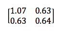
The numbers on the upper left and lower right represent the variance of the x and y variables, respectively, while the identical numbers on the lower left and upper right represent the covariance between x and y. Because of that identity, such matrices are known as symmetrical. As you can see, the covariance is positive, since the graph near the top of the PCA section points up and to the right.

If two variables increase and decrease together (a line going up and to the right), they have a positive covariance, and if one decreases while the other increases, they have a negative covariance (a line going down and to the right).

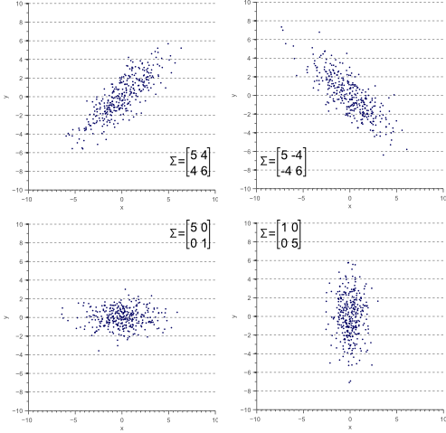
(Credit: Vincent Spruyt)

Notice that when one variable or the other doesn’t move at all, and the graph shows no diagonal motion, there is no covariance whatsoever. Covariance answers the question: do these two variables dance together? If one remains null while the other moves, the answer is no.

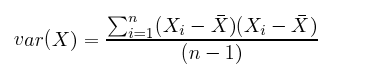
Also, in the equation below, you’ll notice that there is only a small difference between covariance and variance.

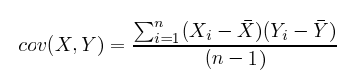
vs.

The great thing about calculating covariance is that, in a high-dimensional space where you can’t eyeball intervariable relationships, you can know how two variables move together by the positive, negative or non-existent character of their covariance. (Correlation is a kind of normalized covariance, with a value between -1 and 1.)

To sum up, the covariance matrix defines the shape of the data. Diagonal spread along eigenvectors is expressed by the covariance, while x-and-y-axis-aligned spread is expressed by the variance.

Causality has a bad name in statistics, so take this with a grain of salt:

While not entirely accurate, it may help to think of each component as a causal force in the Dutch basketball player example above, with the first principal component being age; the second possibly gender; the third nationality (implying nations’ differing healthcare systems), and each of those occupying its own dimension in relation to height. Each acts on height to different degrees. You can read covariance as traces of possible cause.

Change of Basis

Because the eigenvectors of the covariance matrix are orthogonal to each other, they can be used to reorient the data from the x and y axes to the axes represented by the principal components. You re-base the coordinate system for the dataset in a new space defined by its lines of greatest variance.

The x and y axes we’ve shown above are what’s called the basis of a matrix; that is, they provide the points of the matrix with x, y coordinates. But it is possible to recast a matrix along other axes; for example, the eigenvectors of a matrix can serve as the foundation of a new set of coordinates for the same matrix. Matrices and vectors are animals in themselves, independent of the numbers linked to a specific coordinate system like x and y.

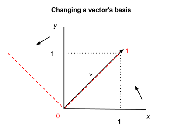
In the graph above, we show how the same vector v can be situated differently in two coordinate systems, the x-y axes in black, and the two other axes shown by the red dashes. In the first coordinate system, v = (1,1), and in the second, v = (1,0), but v itself has not changed. Vectors and matrices can therefore be abstracted from the numbers that appear inside the brackets.

This has profound and almost spiritual implications, one of which is that there exists no natural coordinate system, and mathematical objects in n-dimensional space are subject to multiple descriptions. (Changing matrices’ bases also makes them easier to manipulate.)

A change of basis for vectors is roughly analogous to changing the base for numbers; i.e. the quantity nine can be described as 9 in base ten, as 1001 in binary, and as 100 in base three (i.e. 1, 2, 10, 11, 12, 20, 21, 22, 100 <– that is “nine”). Same quantity, different symbols; same vector, different coordinates.

Entropy & Information Gain

In information theory, the term entropy refers to information we don’t have (normally people define “information” as what they know, and jargon has triumphed once again in turning plain language on its head to the detriment of the uninitiated). The information we don’t have about a system, its entropy, is related to its unpredictability: how much it can surprise us.

If you know that a certain coin has heads embossed on both sides, then flipping the coin gives you absolutely no information, because it will be heads every time. You don’t have to flip it to know. We would say that two-headed coin contains no information, because it has no way to surprise you.

A balanced, two-sided coin does contain an element of surprise with each coin toss. And a six-sided die, by the same argument, contains even more surprise with each roll, which could produce any one of six results with equal frequency. Both those objects contain information in the technical sense.

Now let’s imagine the die is loaded, it comes up “three” on five out of six rolls, and we figure out the game is rigged. Suddenly the amount of surprise produced with each roll by this die is greatly reduced. We understand a trend in the die’s behavior that gives us greater predictive capacity.

Understanding the die is loaded is analogous to finding a principal component in a dataset. You simply identify an underlying pattern.

That transfer of information, from what we don’t know about the system to what we know, represents a change in entropy. Insight decreases the entropy of the system. Get information, reduce entropy. This is information gain. And yes, this type of entropy is subjective, in that it depends on what we know about the system at hand. (Fwiw, information gain is synonymous with Kullback-Leibler divergence, which we explored briefly in this tutorial on restricted Boltzmann machines.)

So each principal component cutting through the scatterplot represents a decrease in the system’s entropy, in its unpredictability.

It so happens that explaining the shape of the data one principal component at a time, beginning with the component that accounts for the most variance, is similar to walking data through a decision tree. The first component of PCA, like the first if-then-else split in a properly formed decision tree, will be along the dimension that reduces unpredictability the most.

1) In some cases, matrices may not have a full set of eigenvectors; they can have at most as many linearly independent eigenvectors as their respective order, or number of dimensions.

Other Posts on the Pathmind Wiki

• Deep Neural Networks
• Recurrent Neural Networks (RNNs) and LSTMs
• Word2vec and Neural Word Embeddings
• Convolutional Neural Networks (CNNs) and Image Processing
• Accuracy, Precision and Recall
• Attention Mechanisms and Transformers
• Graph Analytics and Deep Learning
• Symbolic Reasoning and Machine Learning
• Markov Chain Monte Carlo, AI and Markov Blankets
• Deep Reinforcement Learning
• Generative Adversarial Networks (GANs)
• AI vs Machine Learning vs Deep Learning
• Multilayer Perceptrons (MLPs)