Deep Autoencoders

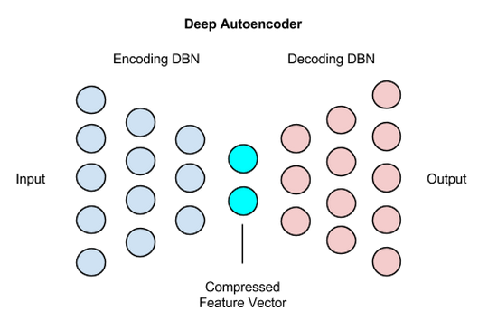
A deep autoencoder is composed of two, symmetrical deep-belief networks that typically have four or five shallow layers representing the encoding half of the net, and second set of four or five layers that make up the decoding half.

The layers are restricted Boltzmann machines, the building blocks of deep-belief networks, with several peculiarities that we’ll discuss below. Here’s a simplified schema of a deep autoencoder’s structure, which we’ll explain below.

Processing the benchmark dataset MNIST, a deep autoencoder would use binary transformations after each RBM. Deep autoencoders can also be used for other types of datasets with real-valued data, on which you would use Gaussian rectified transformations for the RBMs instead.

Encoding Input Data

Let’s sketch out an example encoder:

 784 (input) ----> 1000 ----> 500 ----> 250 ----> 100 -----> 30

If, say, the input fed to the network is 784 pixels (the square of the 28x28 pixel images in the MNIST dataset), then the first layer of the deep autoencoder should have 1000 parameters; i.e. slightly larger.

This may seem counterintuitive, because having more parameters than input is a good way to overfit a neural network.

In this case, expanding the parameters, and in a sense expanding the features of the input itself, will make the eventual decoding of the autoencoded data possible.

This is due to the representational capacity of sigmoid-belief units, a form of transformation used with each layer. Sigmoid belief units can’t represent as much as information and variance as real-valued data. The expanded first layer is a way of compensating for that.

The layers will be 1000, 500, 250, 100 nodes wide, respectively, until the end, where the net produces a vector 30 numbers long. This 30-number vector is the last layer of the first half of the deep autoencoder, the pretraining half, and it is the product of a normal RBM, rather than an classification output layer such as Softmax or logistic regression, as you would normally see at the end of a deep-belief network.

Decoding Representations

Those 30 numbers are an encoded version of the 28x28 pixel image. The second half of a deep autoencoder actually learns how to decode the condensed vector, which becomes the input as it makes its way back.

The decoding half of a deep autoencoder is a feed-forward net with layers 100, 250, 500 and 1000 nodes wide, respectively. Layer weights are initialized randomly.

	784 (output) <---- 1000 <---- 500 <---- 250 <---- 30

The decoding half of a deep autoencoder is the part that learns to reconstruct the image. It does so with a second feed-forward net which also conducts back propagation. The back propagation happens through reconstruction entropy.

Training Nuances

At the stage of the decoder’s backpropagation, the learning rate should be lowered, or made slower: somewhere between 1e-3 and 1e-6, depending on whether you’re handling binary or continuous data, respectively.

Use Cases

Image Search

As we mentioned above, deep autoencoders are capable of compressing images into 30-number vectors.

Image search, therefore, becomes a matter of uploading an image, which the search engine will then compress to 30 numbers, and compare that vector to all the others in its index.

Vectors containing similar numbers will be returned for the search query, and translated into their matching image.

Data Compression

A more general case of image compression is data compression. Deep autoencoders are useful for semantic hashing, as discussed in this paper by Geoff Hinton.

Topic Modeling & Information Retrieval (IR)

Deep autoencoders are useful in topic modeling, or statistically modeling abstract topics that are distributed across a collection of documents.

This, in turn, is an important step in question-answer systems like Watson.

In brief, each document in a collection is converted to a Bag-of-Words (i.e. a set of word counts) and those word counts are scaled to decimals between 0 and 1, which may be thought of as the probability of a word occurring in the doc.

The scaled word counts are then fed into a deep-belief network, a stack of restricted Boltzmann machines, which themselves are just a subset of feedforward-backprop autoencoders. Those deep-belief networks, or DBNs, compress each document to a set of 10 numbers through a series of sigmoid transforms that map it onto the feature space.

Each document’s number set, or vector, is then introduced to the same vector space, and its distance from every other document-vector measured. Roughly speaking, nearby document-vectors fall under the same topic.

For example, one document could be the “question” and others could be the “answers,” a match the software would make using vector-space measurements.